If you’re not into coding, go to settings and turn off notifications for “AI & Python” (leave the rest the same to keep receiving my other emails)
If you’re learning Python and would like to develop a machine learning model then a library that you want to seriously consider is scikit-learn. Scikit-learn (also known as sklearn) is a machine learning library used in Python that provides many unsupervised and supervised learning algorithms.
In this simple guide, we’re going to create a machine learning model that will predict whether a movie review is positive or negative. This is known as binary text classification and will help us explore the scikit-learn library while building a basic machine learning model from scratch. Below are the concepts we’re going to learn in this guide.
<strong>Table of Contents
</strong>1. The Dataset and The Problem to Solve
2. Preparing The Data
 - Reading the dataset
 - Dealing with Imbalanced Classes
 - Splitting data into train and test set
3. Text Representation (Bag of Words)
 - CountVectorizer
 - Term Frequency, Inverse Document Frequency (TF-IDF)
 - Turning our text data into numerical vectors
4. Model Selection
 - Supervised vs Unsupervised learning
 - Support Vector Machines (SVM)
 - Decision Tree
 - Naive Bayes
 - Logistic Regression
5. Model Evaluation
 - Mean Accuracy
 - F1 Score
 - Classification report
 - Confusion Matrix
6. Tuning the Model
 - GridSearchCV
The Dataset and The Problem to Solve
👉 Dataset: In this guide, we’ll use an IMDB dataset of 50k movie reviews available on Kaggle. The dataset contains 2 columns (review and sentiment) that will help us identify whether a review is positive or negative.
Problem formulation: Our goal is to find which machine learning model is best suited to predict sentiment (output) given a movie review (input).
Preparing The Data
Reading the dataset
After you download the dataset, make sure the file is in the same place where your Python script is located. Then, we’ll read the file using the Pandas library.
<strong>import</strong> pandas <strong>as</strong> pd

df_review = pd.read_csv('IMDB Dataset.csv')
df_review
Note: If you don’t have some of the libraries used in this guide, you can easily install a library with pip on your terminal or command prompt (e.g.,pip install scikit-learn)
The dataset looks like the picture below.

This dataset contains 50000 rows; however, to train our model faster in the following steps, we’re going to take a smaller sample of 10000 rows. This small sample will contain 9000 positive and 1000 negative reviews to make the data imbalanced (so I can teach you undersampling and oversampling techniques in the next step)
We’re going to create this small sample with the following code. The name of this imbalanced dataset will bedf_review_imb
df_positive = df_review[df_review['sentiment']=='positive'][:9000]
df_negative = df_review[df_review['sentiment']=='negative'][:1000]

df_review_imb = pd.concat([df_positive, df_negative])
Dealing with Imbalanced Classes
In most cases, you’ll have a large amount of data for one class, and much fewer observations for other classes. This is known as imbalanced data because the number of observations per class is not equally distributed.
Let’s take a look at how our df_review_imb dataset is distributed.

As we can see there are more positive than negative reviews in df_review_imb so we have imbalanced data.
To resample our data we use the imblearn library. You can either undersample positive reviews or oversample negative reviews (you need to choose based on the data you’re working with). In this case, we’ll use the RandomUnderSampler
<strong>from</strong> imblearn.under_sampling <strong>import</strong>  RandomUnderSampler

rus = RandomUnderSampler(random_state=0)
df_review_bal, df_review_bal['sentiment']=rus.fit_resample(df_review_imb[['review']],
                                                           df_review_imb['sentiment'])
df_review_bal
First, we create a new instance of RandomUnderSampler (rus), we add random_state=0 just to control the randomization of the algorithm. Then we resample the imbalanced dataset df_review_imb by fitting rus with rus.fit_resample(x, y) where “x” contains the data which have to be sampled and “y” corresponds to labels for each sample in “x”.
After this, x and y are balanced and we’ll store it in a new dataset named df_review_bal. We can compare the imbalanced and balanced dataset with the following code.
IN [0]: print(df_review_imb.value_counts(‘sentiment’))
        print(df_review_bal.value_counts(‘sentiment’))

OUT [0]:positive    9000
        negative    1000

        negative    1000
        positive    1000
As we can see, now our dataset is equally distributed.
Note 1: If you get the following error when using the RandomUnderSampler
IndexError: only integers, slices (`:`), ellipsis (`…`), numpy.newaxis (`None`) and integer or boolean arrays are valid indices
You can use an alternative to RandomUnderSampler. Try the code below:
# option 2
length_negative = len(df_review_imb[df_review_imb['sentiment']=='negative'])
df_review_positive = df_review_imb[df_review_imb['sentiment']=='positive'].sample(n=length_negative)
df_review_non_positive = df_review_imb[~(df_review_imb['sentiment']=='positive')]

df_review_bal = pd.concat([
    df_review_positive, df_review_non_positive
])
df_review_bal.reset_index(drop=True, inplace=True)
df_review_bal['sentiment'].value_counts()
The df_review_bal dataframe should have now 1000 positive and negative reviews as shown above.
Splitting data into train and test set
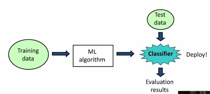
Before we work with our data, we need to split it into a train and test set. The train dataset will be used to fit the model, while the test dataset will be used to provide an unbiased evaluation of a final model fit on the training dataset.
We’ll use sklearn’s train_test_split to do the job. In this case, we set 33% to the test data.
<strong>from</strong> sklearn.model_selection <strong>import</strong> train_test_split

train, test = train_test_split(df_review_bal, test_size=0.33, random_state=42)
Now we can set the independent and dependent variables within our train and test set.
train_x, train_y = train['review'], train['sentiment']
test_x, test_y = test['review'], test['sentiment']
Let’s see what each of them mean:
-
train_x: Independent variables (review) that will be used to train the model. Since we specified
test_size = 0.33, 67% of observations from the data will be used to fit the model. -
train_y: Dependent variables (sentiment) or target label that need to be predicted by this model.
-
test_x: The remaining
33%of independent variables that will be used to make predictions to test the accuracy of the model. -
test_y: Category labels that will be used to test the accuracy between actual and predicted categories.
Text Representation (Bag of Words)
Classifiers and learning algorithms expect numerical feature vectors rather than raw text documents. This is why we need to turn our movie review text into numerical vectors. There are many text representation techniques such as one-hot encoding, bag of words, and wor2vec.
For this simple, we’ll use bag of words (BOW) since we care about the frequency of the words in text reviews; however, the order of words is irrelevant. Two common ways to represent bag of words are CountVectorizer and Term Frequency, Inverse Document Frequency (TF-IDF). Before we choose any of them, I’ll give you an easy-to-understand demonstration of how they work.
CountVectorizer
The CountVectorizer gives us the frequency of occurrence of words in a document. Let’s consider the following sentences.
review = [“I love writing code in Python. I love Python code”,
          “I hate writing code in Java. I hate Java code”]
The representation with CountVectorizer will look like this,
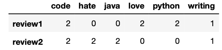
As you can see the numbers inside the matrix represent the number of times each word was mentioned in each review. Words like “love,” “hate,” and “code” have the same frequency (2) in this example.
Term Frequency, Inverse Document Frequency (TF-IDF)
The TF-IDF computes “weights” that represents how important a word is to a document in a collection of documents (aka corpus). The TF-IDF value increases proportionally to the number of times a word appears in the document and is offset by the number of documents in the corpus that contain the word.
The representation with TF-IDF will look like the picture below for the same text we used before.
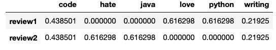
Unlike, the previous example the word “code” doesn’t have the same weight as the words “love” or “hate.” This happens because “code” appears in both reviews; therefore, its weight decreased.
Turning our text data into numerical vectors
In our original dataset, we want to identify unique/representative words for positive reviews and negative reviews, so we’ll choose the TF-IDF. To turn text data into numerical vectors with TF-IDF, we write the following code.
<strong>from</strong> sklearn.feature_extraction.text <strong>import</strong> TfidfVectorizer

tfidf = TfidfVectorizer(stop_words='english')
train_x_vector = tfidf.fit_transform(train_x)
train_x_vector

Out[0]: <1340x20625 sparse matrix of type '<class 'numpy.float64'>'
	with 118834 stored elements in Compressed Sparse Row format>
In the code above, we create a new instance of TfidfVectorizer(tfidf), we removed English stopwords and then fit (finds the internal parameters of a model) and transform (applies the parameters to the data) the train_x (text reviews)
The train_x_vector we just created is a sparse matrix with a shape of 1340 reviews and 20625 words (whole vocabulary used in the reviews). You can display this matrix like the pictures I used in the examples above with the following code
pd.DataFrame.sparse.from_spmatrix(train_x_vector,
                                  index=train_x.index,
                                  columns=tfidf.get_feature_names())
However, keep in mind that you’ll find lots of ‘0’ since its a sparse matrix with 1340×20625 elements where only 118834 elements are different from “0”
Finally, let’s also transform the test_x_vector, so we can test the accuracy of the model later (we don’t need to fit tfidf again since we already did it with the training data.)
test_x_vector = tfidf.transform(test_x)Model Selection
Now that we have numerical data, we can experiment with different machine learning models and evaluate their accuracy.
Supervised vs Unsupervised learning
Machine learning algorithms are divided between supervised learning and unsupervised learning. In the first, models are trained using labeled data, while in the second patterns are inferred from the unlabeled input data.
In our example, our input (review) and output (sentiment) are clearly identified, so we can say we have labeled input and output data; therefore, we’re dealing with supervised learning. Two common types of supervised learning algorithms are Regression and Classification.
-
Regression: They’re used to predict continuous values such as price, salary, age, etc
-
Classification: They’re used to predict discrete values such as male/female, spam/not spam, positive/negative, etc.
That said, it’s now evident that we should use classification algorithms. We will benchmark the following four classification models.
Note: I’m going to leave the theory behind each model for you to research. I’m going to focus on the code and how we choose the best model based on the scores.
Support Vector Machines (SVM)
To fit an SVM model, we need to introduce the input (text reviews as numerical vectors) and output (sentiment)
<strong>from</strong> sklearn.svm <strong>import</strong> SVC

svc = SVC(kernel=’linear’)
svc.fit(train_x_vector, train_y)
After fitting svc we can predict whether a review is positive or negative with the .predict() method.
print(svc.predict(tfidf.transform(['A good movie'])))
print(svc.predict(tfidf.transform(['An excellent movie'])))
print(svc.predict(tfidf.transform(['I did not like this movie at all'])))
If you run the code above, you’ll obtain that the first and second reviews are positive, while the third is negative.
Decision Tree
To fit a decision tree model, we need to introduce the input (text reviews as numerical vectors) and output (sentiment)
<strong>from</strong> sklearn.tree <strong>import</strong> DecisionTreeClassifier

dec_tree = DecisionTreeClassifier()
dec_tree.fit(train_x_vector, train_y)
Naive Bayes
To fit a Naive Bayes model, we need to introduce the input (text reviews as numerical vectors) and output (sentiment)
<strong>from</strong> sklearn.naive_bayes <strong>import</strong> GaussianNB

gnb = GaussianNB()
gnb.fit(train_x_vector.toarray(), train_y)
Logistic Regression
To fit a Logistic Regression model, we need to introduce the input (text reviews as numerical vectors) and output (sentiment)
<strong>from</strong> sklearn.linear_model <strong>import</strong> LogisticRegression

log_reg = LogisticRegression()
log_reg.fit(train_x_vector, train_y)
Model Evaluation
In this section, we’ll see traditional metrics used to evaluate our models.
Mean Accuracy
To obtain the mean accuracy of each model, just use the .score method with the test samples and true labels as shown below.
# svc.score('Test samples', 'True labels')

svc.score(test_x_vector, test_y)
dec_tree.score(test_x_vector, test_y)
gnb.score(test_x_vector.toarray(), test_y)
log_reg.score(test_x_vector, test_y)
After printing each of them, we obtain the mean accuracy.
SVM: 0.84
Decision tree: 0.64
Naive Bayes: 0.63
Logistic Regression: 0.83
SVM and Logistic Regression perform better than the other two classifiers, with SVM having a slight advantage (84% of accuracy). To show how the other metrics work, we’ll focus only on SVM.
F1 Score
F1 Score is the weighted average of Precision and Recall. Accuracy is used when the True Positives and True negatives are more important while F1-score is used when the False Negatives and False Positives are crucial. Also, F1 takes into account how the data is distributed, so it’s useful when you have data with imbalance classes.
F1 score is calculated with the following formula. (If you don’t know what precision and recall means, check this great explanation on stackoverflow)
F1 Score = 2*(Recall * Precision) / (Recall + Precision)

F1 score reaches its best value at 1 and worst score at 0.
To obtain the F1 score, we need the true labels and predicted labelsf1_score(y_true, y_pred)
<strong>from</strong> sklearn.metrics <strong>import</strong> f1_score

f1_score(test_y, svc.predict(test_x_vector),
         labels=['positive', 'negative'],
         average=None)
The score obtained for positive labels is 0.84, while negative labels is 0.83.
Classification report
We can also build a text report showing the main classification metrics that include those calculated before. To obtain the classification report, we need the true labels and predicted labels classification_report(y_true, y_pred)
<strong>from</strong> sklearn.metrics <strong>import</strong> classification_report

print(classification_report(test_y,
                            svc.predict(test_x_vector),
                            labels=['positive', 'negative']))
After printing, we obtain the following report.
               precision    recall  f1-score   support

    positive       0.83      0.87      0.85       335
    negative       0.85      0.82      0.83       325

    accuracy                           0.84       660
   macro avg       0.84      0.84      0.84       660
weighted avg       0.84      0.84      0.84       660
As we can see, the accuracy and f1-score are the same as those previously calculated.
Confusion Matrix
A confusion matrix) is a table that allows visualization of the performance of an algorithm. This table typically has two rows and two columns that report the number of false positives, false negatives, true positives, and true negatives (check the graph in this link in case you don’t understand these terms)
To obtain the confusion matrix, we need the true labels and predicted labels.
<strong>from</strong> sklearn.metrics <strong>import</strong> confusion_matrix

conf_mat = confusion_matrix(test_y,
                            svc.predict(test_x_vector),
                            labels=['positive', 'negative'])
After running the code below, we’ll obtain the following array as output.
array([[290,  45],
       [ 60, 265]])
To understand what that means check this picture below.
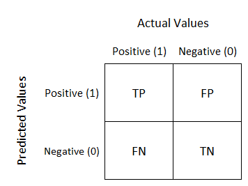
As you can see, each element of the array represents one of the four squares in the confusion matrix (e.g., our model detected 290 true positives)
Tuning the Model
Finally, it’s time to maximize our model’s performance.
GridSearchCV
This is technique consists of an exhaustive search on specified parameters in order to obtain the optimum values of hyperparameters. To do so, we write the following code.
<strong>from</strong> sklearn.model_selection <strong>import</strong> GridSearchCV

# set the parameters
parameters = {‘C’: [1,4,8,16,32] ,’kernel’:[‘linear’, ‘rbf’]}
svc = SVC()
svc_grid = GridSearchCV(svc,parameters, cv=5)

svc_grid.fit(train_x_vector, train_y)
As you can see the code it’s not so different from the one we wrote to fit the SVM model; however, now we specified some parameters to obtain the optimum model.
After fitting the model, we obtain the best score, parameters, and estimators with the following code.
IN [0]: print(svc_grid.best_params_)
        print(svc_grid.best_estimator_)

OUT [0]: {'C': 1, 'kernel': 'linear'}
         SVC(C=1, kernel='linear')
That’s it! Now you’re ready to create your own machine learning model using sklearn!
👉 Code: All the code written in this guide can be found on my Github.